hfr is an R package that implements a novel graph-based regularized regression estimator: the Hierarchical Feature Regression (HFR). The method mobilizes insights from the domains of machine learning and graph theory to estimate robust parameters for a linear regression, constructing a supervised feature graph that decomposes parameters along its edges. The graph adjusts first for common variation and successively incorporates idiosyncratic patterns into the fitting process.

The result is group shrinkage of the parameters, where the extent of shrinkage is governed by a hyperparameter kappa that represents the size of the feature graph. At kappa = 1 the regression is unregularized resulting in OLS parameters. At kappa < 1 the graph is shrunken, reducing the effective model size and regularizing the regression.

Usage: at a glance

Fit a linear regression using simulated data from the glmnet package:

library(hfr)

data("QuickStartExample", package = "glmnet")
data <- QuickStartExample

mod <- hfr(data$x, data$y, kappa = 0.75)
print(mod)

## 
## Call:  hfr(x = data$x, y = data$y, kappa = 0.75) 
## 
##   Df R.squared kappa
## 1 16      0.91  0.75

Cross-validation to select an optimal kappa can be done using cv.hfr. The default in cv.hfr is a 10-fold CV, however, we will pass foldid to use an LOOCV algorithm:

cv <- cv.hfr(data$x, data$y, foldid = 1:nrow(data$x))
mod <- hfr(data$x, data$y, kappa = cv$best_kappa)

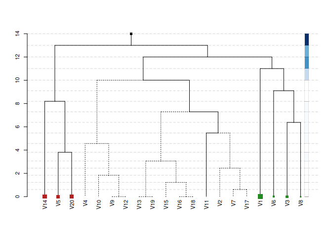
The HFR offers useful tools for the visual exploration of the effect structure in the data. The package includes a custom dendrogram visualizing the optimal feature graph. See ?plot.hfr for details:

par(family = "sans", cex = 0.7)
plot(mod, confidence_level = 0.95, max_leaf_size = 2, show_details = FALSE)

The plot displays the optimal supervised feature graph. The size of the tree represents the effective model size — in this case reducing the model from p = 20 variables to an effective size of 14 variables. The plot conveys a wealth of additional information:

• Adjacent variables that are merged low in the graph have a similar conditional explanatory effect on y
• The vertical distance between levels indicates the weight of the levels in the regression
• The size of the leaf nodes represents the coefficient size and the color represents the sign
• Dashed edges are statistically insignificant (see ?se.avg for standard errors)
• Darker hues in the sidebar signify a higher contribution of that level to total explained variance

Standard functions such as coef, predict and print can be used to interact with fitted hfr or cv.hfr objects.

Installation

# CRAN
install.packages("hfr")

# Latest Dev version
devtools::install_github("https://github.com/jpfitzinger/hfr")

References

Pfitzinger, J. (2024). Cluster Regularization via a Hierarchical Feature Regression. Econometrics and Statistics (in press). https://doi.org/10.1016/j.ecosta.2024.01.003.